Abstract

摘要

This paper develops a systematic framework for assessing U.S. sovereign debt sustainability, proceeding from the problem statement and theoretical foundations to modeling, data, analysis, and conclusions. It uses the latest publicly available data for 2026 to construct mechanism-based projections of the U.S. debt trajectory.

本文建立了一个评估美国主权债务可持续性的系统性框架，从问题陈述和理论基础到建模、数据、分析和结论逐步展开。文章使用2026年最新公开数据，构建了基于机制的美国债务轨迹预测。

The paper advances three principal arguments. First, the key test of debt sustainability is the differential between the interest rate and the rate of economic growth, or r − g. In 2026, the U.S. r − g differential turned positive for the first time since 2008, reaching 0.51 percentage point and signaling the loss of a previously self-stabilizing dynamic. Second, the basic single-sector model (Equations 1–5), together with the IMF's broader risk framework (Equations 6–12), indicates that the primary surplus required to stabilize debt under the current fiscal parameters is positive—0.71% of GDP—while the actual primary balance is a deficit of 2.6% of GDP. This implies a fiscal gap of approximately 3.3 percentage points. Third, scenario simulations suggest that, if policy and interest-rate conditions remain unchanged, debt held by the public could reach approximately 198% of GDP by 2055 under current-policy assumptions, compared with 156% under the Congressional Budget Office (CBO) baseline. Both trajectories place debt in the divergence region of the stability diagram.

本文提出三个主要论点。第一，债务可持续性的关键检验是利率与经济增长率之间的差值，即 r − g。2026年，美国 r − g 差值自2008年以来首次转为正值，达到0.51个百分点，标志着原有自动稳定机制的丧失。第二，基本单部门模型（方程1–5）与 IMF 更广泛的风险框架（方程6–12）表明，在当前财政参数下稳定债务所需的基本盈余为正值——占 GDP 的0.71%——而实际基本余额为 GDP 的2.6%赤字。这意味着约3.3个百分点的财政缺口。第三，情景模拟表明，如果政策和利率条件保持不变，在当前政策假设下，到2055年公众持有的债务可能达到 GDP 的约198%，而 CBO 基线情景下为156%。两种轨迹都将债务置于稳定性图的发散区域。

Beyond the formal models, the paper reviews several relevant concepts in public finance and macroeconomics, including Ricardian equivalence, fiscal and monetary dominance, the safe-asset hypothesis, financial repression, generational accounting and overlapping-generations (OLG) models, fiscal reaction functions, and debt spirals. These concepts help explain why high debt could be sustained during an era of low r − g—and how risks may emerge as that advantage fades.

除了正式模型之外，本文还回顾了公共财政和宏观经济学中的几个相关概念，包括李嘉图等价、财政与货币主导、安全资产假说、金融抑制、代际核算和世代交叠(OLG)模型、财政反应函数以及债务螺旋。这些概念有助于解释为什么在低 r − g 时代可以维持高债务——以及随着这一优势消退，风险如何可能出现。

Keywords:sovereign debt sustainability; r − g framework; intertemporal budget constraint; fiscal dominance; safe assets; IMF Debt Sustainability Analysis (DSA); U.S. Treasury securities

关键词：主权债务可持续性；r-g 框架；跨期预算约束；财政主导；安全资产；IMF 债务可持续性分析(DSA)；美国国债

1. The Question

1. 问题的提出

For much of the past decade, low real borrowing costs helped contain the burden of America's rising debt. As that advantage fades, the arithmetic of debt stabilization is becoming less forgiving—and the choices facing fiscal and monetary policymakers more consequential.

在过去十年的大部分时间里，低实际借贷成本帮助遏制了美国不断上升的债务负担。随着这一优势的消退，债务稳定的算术空间正不断收窄——财政与货币政策制定者面临的选择影响也更为重大。

U.S. federal debt reached a historic high in 2026. According to Federal Reserve Economic Data (FRED), gross federal debt stood at 122.6% of GDP in the first quarter of 2026. On the CBO measure, debt held by the public amounted to 101% of GDP. Both measures are substantially above the IMF's 85% debt benchmark for advanced economies and exceed the 106% peak recorded in 1946, at the end of World War II, on the gross-debt measure.

美国联邦债务在2026年达到历史新高。根据美联储经济数据(FRED)，2026年第一季度联邦总债务占 GDP 的122.6%。按照 CBO 的衡量标准，公众持有的债务占 GDP 的101%。两项指标都大幅高于 IMF 对发达经济体设定的85%债务基准，并且在总债务衡量标准上超过了1946年第二次世界大战结束时创下的106%峰值。

These figures raise three related questions.

这些数字引发了三个相关问题。

First, does high debt necessarily mean that debt is unsustainable? The debt-to-GDP ratio, taken in isolation, is not conclusive. Japan in the 1990s and the United States and United Kingdom after World War II experienced debt ratios well above today's levels without immediately defaulting. What ultimately matters is the debt trajectory: is the ratio converging or diverging?

第一，高债务是否必然意味着债务不可持续？债务与 GDP 的比率单独来看并不具有决定性。20世纪90年代的日本以及二战后的美国和英国都经历了远高于今天水平的债务比率，但并未立即违约。最终重要的是债务轨迹：比率是收敛还是发散？

Second, why could high debt be sustained during the era of low interest rates? From 2009 to 2021, U.S. real interest rates remained below real economic growth for extended periods (r − g < 0). Olivier Blanchard (2019) described the implications as a "low-interest-rate utopia": in such an environment, economic growth itself dilutes the debt burden, allowing the debt ratio to remain stable without active fiscal adjustment. Did this "growth dividend" come to an end in 2026?

第二，为什么在低利率时代可以维持高债务？从2009年到2021年，美国实际利率长期低于实际经济增长率(r − g < 0)。Olivier Blanchard(2019)将这种情况的影响描述为“低利率乌托邦”：在这种环境下，经济增长本身就稀释了债务负担，使债务比率无需主动财政调整即可保持稳定。这种“增长红利”是否在2026年终结？

Third, how can sustainability be rigorously defined and projected? With r − g turning positive and the primary deficit remaining large, how will the debt path evolve? Is there a clearly identifiable stabilization condition, and how far is the United States from meeting it?

第三，如何严格定义和预测可持续性？随着 r − g 转为正值且基本赤字仍然很大，债务路径将如何演变？是否存在明确可识别的稳定条件，美国距离满足该条件有多远？

This paper does not seek to deliver a binary verdict on whether the United States will or will not default. Its objective is to establish a calculable and falsifiable analytical framework and use it to develop a mechanism-based projection of the U.S. debt path from 2026 to 2055.

本文并不试图就美国是否会违约做出二元判断。其目标是建立一个可计算和可证伪的分析框架，并据此构建 2026 年至 2055 年美国债务路径的机制化预测。

2. Theoretical Foundations: The Economics Behind Sovereign-Debt Projections

2. 理论基础：主权债务预测背后的经济学

Projecting sovereign debt is not a matter of simple arithmetic extrapolation. It requires a framework grounded in macroeconomics, public finance, and financial theory. This section reviews the concepts needed to understand the U.S. debt challenge.

预测主权债务不是简单的算术推演问题。它需要一个植根于宏观经济学、公共财政和金融理论的框架。本节回顾了理解美国债务挑战所需的概念。

2.1 The Central Test of Debt Dynamics: The r − g Framework

2.1 债务动态的核心检验：r-g 框架

In his 2019 American Economic Association presidential address, Blanchard argued that when the interest rate is below the growth rate (r < g), a government may be able to roll over its debt indefinitely without corresponding tax increases; debt can, in effect, become approximately self-financing. A change in the sign of r − g is therefore an important early warning signal.

在2019年美国经济学会主席演讲中，Blanchard 认为，当利率低于增长率(r < g)时，政府可能能够无限期展期其债务而无需相应增税；债务实际上可以变得近乎自我融资。因此，r − g 符号的变化是一个重要的早期预警信号。

The simplest test of debt sustainability is the approximate debt-ratio dynamic: Δd ≈ (r − g) × d − s (see Equation 2). When r > g, the debt ratio has a self-reinforcing, "snowball" tendency to rise. When r < g, economic growth dilutes the debt burden and the ratio tends toward self-stabilization.

债务可持续性的最简单检验是近似的债务比率动态：Δd ≈ (r − g) × d − s（见方程2）。当 r > g 时，债务比率具有自我强化的“滚雪球”上升趋势。当 r < g 时，经济增长稀释债务负担，比率趋向自我稳定。

2.2 Ricardian Equivalence and the Limits of Fiscal Adjustment

2.2 李嘉图等价与财政调整的局限

The Ricardian-equivalence proposition, developed by Robert Barro (1974), holds that under ideal conditions—including rational expectations, complete markets, and sufficiently strong intergenerational altruism—debt financing and tax financing have equivalent effects on the real economy. Households anticipate future tax increases and save an amount equal to the debt-financed tax reduction, leaving consumption and interest rates unchanged. Public debt is, in this view, merely "taxation deferred." If the proposition held fully, debt expansion would impose little real cost and sustainability would face few constraints.

由 Robert Barro(1974)提出的李嘉图等价命题认为，在理想条件下——包括理性预期、完全市场和足够强的代际利他主义——债务融资和税收融资对实体经济具有等价效应。家庭预期未来税收增加，并储蓄相当于债务融资减税的金额，使消费和利率保持不变。在这种观点下，公共债务仅仅是“延迟的税收”。如果这一命题完全成立，债务扩张带来的实际成本有限，可持续性将几乎不受约束。

In practice, however, liquidity constraints, short planning horizons, incomplete intergenerational altruism, and financial-market frictions substantially weaken the equivalence (Bernheim, 1989). Public debt therefore creates an intertemporal burden, and fiscal discipline cannot be left to an assumed automatic offset by private saving.

然而在实践中，流动性约束、有限规划期、不完全的代际利他主义以及金融市场摩擦大大削弱了这种等价性(Bernheim, 1989)。因此，公共债务造成了跨期负担，财政纪律不能寄希望于私人储蓄的假定自动抵消。

2.3 Fiscal Dominance and Monetary Dominance

2.3 财政主导与货币主导

Sargent and Wallace (1981) introduced the distinction between fiscal dominance and monetary dominance. Under monetary dominance, the central bank independently controls inflation, while fiscal policy must adjust to remain consistent with that objective. Under fiscal dominance, a substantial fiscal expansion may ultimately pressure the central bank to accommodate government financing needs, making inflation an implicit instrument for reducing the real value of debt.

Sargent 和 Wallace(1981)引入了财政主导和货币主导的区分。在货币主导下，中央银行独立控制通货膨胀，而财政政策必须调整以保持与该目标一致。在财政主导下，大规模财政扩张最终可能迫使中央银行配合政府融资需求，使通货膨胀成为降低债务实际价值的隐性工具。

Leeper (1991) characterized the policy mix in terms of "active" and "passive" policy rules. The United States is currently near the boundary of fiscal dominance: large deficits and a rising debt burden create tensions for monetary policy between containing inflation and preserving fiscal solvency. This helps explain why the inflation outlook can, in turn, affect r and the sustainability of public debt.

Leeper(1991)用“主动”和“被动”政策规则来描述政策组合。美国目前处于财政主导的边界附近：巨额赤字和不断上升的债务负担使货币政策在遏制通胀与维持财政偿付能力之间面临权衡。这有助于解释为什么通胀前景反过来会影响 r 和公共债务的可持续性。

2.4 The Safe-Asset Hypothesis and the Global Saving Glut

2.4 安全资产假说与全球储蓄过剩

Why has the United States been able to sustain relatively low real interest rates despite high debt?

为什么美国尽管债务高企，却能够维持相对较低的实际利率？

On the demand side, the safe-asset hypothesis (Caballero, 2017) and Ben Bernanke's (2005) "global saving glut" are central to the explanation. U.S. Treasury securities serve as core collateral and reserve assets in the global financial system. Emerging-market central banks, pension funds, and insurers have substantial structural demand for them.

从需求方面看，安全资产假说(Caballero, 2017)和 Ben Bernanke(2005)的“全球储蓄过剩”是核心解释。美国国债在全球金融体系中充当核心抵押品和储备资产。新兴市场央行、养老基金和保险公司对其存在大量结构性需求。

This demand compresses term premiums and helps confer on the United States what Gourinchas and Rey (2007) called an "exorbitant privilege": the ability to borrow in its own currency while attracting global demand, thereby lowering funding costs. This is a deeper explanation for the persistence of low r and an important variable in assessing its future path.

这种需求压缩了期限溢价，并赋予美国 Gourinchas 和 Rey(2007)所称的“过度特权”：以本币借款同时吸引全球需求的能力，从而降低融资成本。这是低 r 持续存在的更深层解释，也是评估其未来路径的重要变量。

2.5 Financial Repression, the Inflation Tax, and Historical Deleveraging

2.5 金融抑制、通胀税与历史去杠杆化

When explicit fiscal adjustment is difficult, governments have two additional, less visible channels for reducing the real debt burden.

当显性财政调整困难时，政府还有两条较为隐蔽的渠道可以减轻实际债务负担。

The first is financial repression (Reinhart and Sbrancia, 2011). Through capital controls, directed holdings—for example, requirements or incentives for banks and pension funds to hold low-yielding government bonds—and negative real interest rates, governments can systematically suppress real borrowing costs. This can push r − g below zero and gradually dilute the debt burden. The paper identifies this as a major mechanism behind deleveraging in Europe and the United States from 1945 to 1980.

第一种是金融抑制（Reinhart 和 Sbrancia，2011）。通过资本管制、定向持有——例如要求或激励银行和养老基金持有低收益政府债券——以及负实际利率，政府可以系统性地压制实际借贷成本。这可以将 r − g 推至零以下，并逐渐稀释债务负担。本文将其视为 1945 年至 1980 年欧美去杠杆化背后的主要机制。

The second is the inflation tax. Unexpected inflation reduces the real value of outstanding nominal debt and is economically equivalent to a tax on bondholders. Both mechanisms imply that debt sustainability depends not only on market confidence but also on a government's institutional capacity to sustain negative real interest rates—an important variable in long-term projections.

第二种是通胀税。意外通胀降低了未偿名义债务的实际价值，在经济上相当于对债券持有人征税。这两种机制都意味着债务可持续性不仅取决于市场信心，还取决于政府维持负实际利率的制度能力——这是长期预测中的一个重要变量。

2.6 Generational Accounting and the OLG Perspective

2.6 代际核算与 OLG 视角

In the overlapping-generations (OLG) model developed by Diamond (1965), and in the generational-accounting approach associated with Auerbach and Kotlikoff, public debt is fundamentally a transfer of wealth across generations: consumption by the current generation is supported by the present value of tax burdens borne by future generations.

在 Diamond(1965)开发的世代交叠(OLG)模型中，以及在与 Auerbach 和 Kotlikoff 相关的代际核算方法中，公共债务从根本上是跨代的财富转移：当代的消费由未来几代人承担的税收负担的现值来支撑。

The intertemporal budget constraint, B ≤ Σ sₖ/(1 + r)ᵏ (Equation 5), gives this idea a formal expression. It requires the present value of outstanding debt to be covered by the present value of future primary surpluses. The true boundary of sustainability is therefore not today's debt ratio, but the discounted value of future fiscal surpluses.

跨期预算约束 B ≤ Σ sₖ/(1 + r)ᵏ（方程5）给出了这一思想的形式化表达。它要求未偿债务的现值由未来基本盈余的现值覆盖。因此，可持续性的真正边界不是今天的债务比率，而是未来财政盈余的贴现值。

2.7 Fiscal Reaction Functions, Debt Spirals, and Financing Needs

2.7 财政反应函数、债务螺旋与融资需求

Bohn (1998) sets out a condition for fiscal sustainability: if the primary surplus rises as the debt ratio increases—that is, if s = α + β × d, with β > 0—debt can still be stabilized even when r > g. In other words, the government's fiscal response capacity, rather than the current parameters alone, determines the long-term outcome.

Bohn(1998)提出了财政可持续性的一个条件：如果基本盈余随着债务比率的增加而上升——即如果 s = α + β × d，其中 β > 0——即使在 r > g 时债务仍然可以稳定。换句话说，政府的财政反应能力，而不仅仅是当前参数，决定了长期结果。

If the fiscal reaction function breaks down—for example, because policy becomes politicized or procyclical, or because β ≤ 0—the economy may enter a debt spiral: higher r leads to higher interest expense, which widens the deficit, increases debt, raises the risk premium, and pushes r higher still. Annual gross financing needs, defined as the deficit plus maturing debt that must be refinanced, measure rollover risk. The paper places this U.S. indicator at more than 20% of GDP, making it a useful gauge of short-term vulnerability.

如果财政反应函数失效——例如，因为政策变得政治化或顺周期，或者因为 β ≤ 0——经济可能进入债务螺旋：更高的 r 导致更高的利息支出，这扩大了赤字，增加了债务，提高了风险溢价，并进一步推高 r。年度总融资需求，定义为赤字加上必须再融资的到期债务，衡量展期风险。本文估计美国该指标超过 GDP 的 20%，使其成为短期脆弱性的有用指标。

3. Analytical Models: From a Basic Single-Sector Model to the IMF's Multi-Risk Framework

3. 分析模型：从基本单部门模型到 IMF 多风险框架

Theory must be translated into a model that can be calculated. This paper uses a two-tier framework: a basic single-sector model to capture the core mechanism, and the IMF Debt Sustainability Analysis (DSA) framework to incorporate an open economy and contingent risks.

理论必须转化为可计算的模型。本文使用两层框架：一个基本单部门模型来捕捉核心机制，以及 IMF 债务可持续性分析(DSA)框架来纳入开放经济和或有风险。

3.1 The Basic Model (Equations 1–5)

3.1 基本模型（方程1–5）

The single-sector model decomposes changes in the debt ratio into three forces: the interest-rate effect, the growth effect, and fiscal discipline.

单部门模型将债务比率的变化分解为三种力量：利率效应、增长效应和财政纪律。

Equation 2 is the paper's central diagnostic. When r − g is positive, the debt ratio rises each year by approximately (r − g) × d even if the primary balance is zero. Equation 3 identifies the steady-state primary surplus needed to anchor a given debt ratio and provides a direct measure of the fiscal gap. Equation 5 establishes the hard constraint from a present-value perspective.

方程2是本文的核心诊断工具。当 r − g 为正时，即使基本余额为零，债务比率每年也会增加约 (r − g) × d。方程3确定了锚定给定债务比率所需的稳态基本盈余，并提供了财政缺口的直接衡量标准。方程5从现值角度建立了硬约束。

3.2 The IMF DSA Extension (Equations 6–12)

3.2 IMF DSA 扩展（方程6–12）

The basic model assumes a closed economy, a single currency, and no contingent risks. The IMF's 2022 Sovereign Risk and Debt Sustainability Framework (SRDSF) adds several dimensions:

基本模型假设封闭经济、单一货币且无或有风险。IMF 2022年主权风险和债务可持续性框架(SRDSF)增加了几个维度：

For the United States, the foreign-currency share of public debt is very small, and the dollar's reserve-currency status limits the relevance of the exchange-rate channels in Equations 6–9. Contingent liabilities, however—including implicit guarantees of the kind associated with Fannie Mae and Freddie Mac, as well as fiscal gaps in pensions and health programs—and stock-flow adjustments under Equation 11 remain potential sources of upward pressure on debt.

对于美国而言，公共债务的外币份额非常小，美元的储备货币地位限制了方程6–9中汇率渠道的相关性。然而，或有负债——包括与房利美、房地美（Fannie Mae、Freddie Mac）相关的隐性担保，以及养老金和医疗计划中的财政缺口——以及方程11下的存量—流量调整，仍然是债务上行压力的潜在来源。

3.3 The Intellectual Lineage of the Equations

3.3 方程的知识谱系

The twelve equations are not independent inventions. They are a progressive synthesis of established work across four fields: macroeconomics, public finance, finance, and mathematics.

这十二个方程不是独立发明。它们是跨越四个领域——宏观经济学、公共财政、金融学和数学——的既有研究成果的递进式综合。

4. Data Sources and Calibration of Key Variables for 2026

4. 2026年数据来源与关键变量校准

Model parameters must be calibrated using authoritative data. This paper draws on four public sources and uses the latest available 2026 observations to establish its baseline scenario.

模型参数必须使用权威数据进行校准。本文依据四个公开来源，使用2026年可获得的最新观测数据建立基线情景。

4.1 Authoritative Data Sources

4.1 权威数据来源

FRED (Federal Reserve Bank of St. Louis):the 10-year Treasury Inflation-Protected Securities (TIPS) real yield, DFII10; real GDP, GDPC1; and gross federal debt as a share of GDP, GFDEGDQ188S.

FRED（圣路易斯联邦储备银行）：10年期通胀保值国债（TIPS）实际收益率，DFII10；实际 GDP，GDPC1；以及联邦总债务占 GDP 的比重，GFDEGDQ188S。

Bureau of Economic Analysis (BEA):real GDP growth, reported in the paper as 2.95% in 2024, 2.34% in 2025, and 1.66% in 2026.

经济分析局(BEA)：实际 GDP 增长率，本文报告为2024年2.95%，2025年2.34%，2026年1.66%。

Congressional Budget Office (CBO):debt held by the public as a share of GDP, the primary deficit, net interest costs, and long-term projections for 2025–2055.

国会预算办公室(CBO)：公众持有的债务占 GDP 的比重、基本赤字、净利息成本，以及2025–2055年的长期预测。

International Monetary Fund (IMF):the 2022 SRDSF and Working Paper 2022/123, which provide debt and gross-financing-need benchmarks for advanced and emerging-market economies.

国际货币基金组织(IMF)：2022年 SRDSF 和工作论文2022/123，提供发达经济体和新兴市场经济体的债务和总融资需求基准。

4.2 Calibration of Key Variables for 2026

4.2 2026年关键变量校准

4.3 Differences in Definitions and Comparability

4.3 定义差异与可比性

U.S. debt is commonly reported on both a gross-debt and a debt-held-by-the-public basis. The two measures differ by approximately 20 percentage points. Gross debt includes intragovernmental holdings, such as Treasury securities held by Social Security trust funds; debt held by the public more directly reflects the government's market financing requirements. The IMF benchmark uses general-government debt, so comparisons across definitions require care. Unless otherwise noted, this paper uses the CBO measure of debt held by the public for its projections, consistent with the long-term forecast series. The 122.6% gross-debt figure is used for historical comparisons.

美国债务通常以总债务和公众持有债务两种方式报告。两项指标相差约20个百分点。总债务包括政府内部持有，如社会保障信托基金持有的国债；公众持有的债务更直接地反映了政府的市场融资需求。IMF 基准使用的是一般政府债务，因此跨定义的比较需要谨慎。除非另有说明，本文使用 CBO 的公众持有债务指标进行预测，与长期预测序列一致。122.6%的总债务数字用于历史比较。

5. Projections and Analysis

5. 预测与分析

Applying the calibrated 2026 parameters to the models produces the following findings. All scenarios are constant-parameter mechanism simulations, not official forecasts. Their purpose is to illustrate debt dynamics under different combinations of policy and interest-rate assumptions.

将校准的2026年参数应用于模型，得出以下发现。所有情景都是恒定参数机制模拟，而非官方预测。其目的是说明不同政策和利率假设组合下的债务动态。

5.1 The Debt Ratio Has Moved Beyond Key Benchmarks and Continues to Rise

5.1 债务比率已超越关键基准并持续上升

According to the CBO long-term projection cited in this paper, debt held by the public follows this path as a share of GDP: 101% in 2026, 109% in 2030, 118% in 2035, 132% in 2040, 144% in 2045, 150% in 2050, and 156% in 2055. The ratio remains above the IMF's 85% benchmark throughout and is projected to exceed the World War II peak of 107% on the debt-held-by-the-public measure around 2029. The ratio rises throughout the 30-year projection horizon, with no sign of automatic convergence.

根据本文引用的 CBO 长期预测，公众持有的债务占 GDP 的比重路径如下：2026年101%，2030年109%，2035年118%，2040年132%，2045年144%，2050年150%，2055年156%。该比率始终高于 IMF 的85%基准，预计在2029年左右将超过二战时期107%的峰值（按公众持有债务衡量）。该比率在30年预测期内持续上升，没有自动收敛的迹象。

5.2 A Positive r − g: The Loss of a Self-Stabilizing Mechanism

5.2 正的 r − g：自动稳定机制的丧失

The historical series for the real interest rate minus real GDP growth shows a pronounced turning point:

实际利率减去实际 GDP 增长率的历史序列显示出明显的转折点：

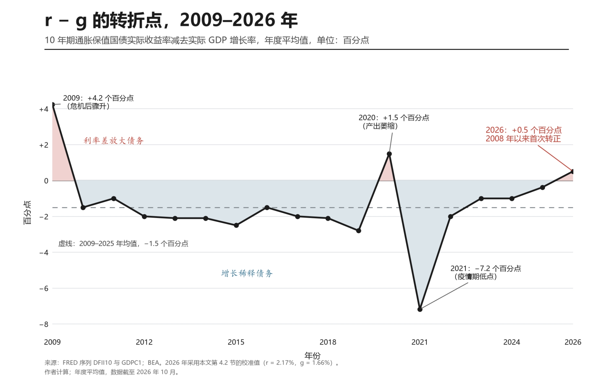
2009: +4.24 percentage points (a brief post-crisis episode); 2012: −2.0 points; 2015: −2.5 points; 2019: −2.8 points; 2021: −7.18 points (low rates during the post-pandemic rebound); 2023: −1.0 point; 2025: −0.38 point; and 2026: +0.51 point.

2009年：+4.24个百分点（危机后的短暂时期）；2012年：−2.0点；2015年：−2.5点；2019年：−2.8点；2021年：−7.18点（疫情后反弹期间的低利率）；2023年：−1.0点；2025年：−0.38点；以及2026年：+0.51点。

This suggests that the United States has exited the r < g "growth-dividend" period that began after 2008. Debt dynamics are shifting from being growth-led to being interest-rate-led. Stabilizing the debt ratio can no longer be treated as something that happens without fiscal effort; it now requires a positive primary surplus. This is the starting point for the paper's divergence assessment.

这表明美国已经退出了2008年后开始的 r < g “增长红利”时期。债务动态正在从增长主导转向利率主导。稳定债务比率不再能依靠自动机制实现；现在需要正的基本盈余。这是本文发散评估的起点。

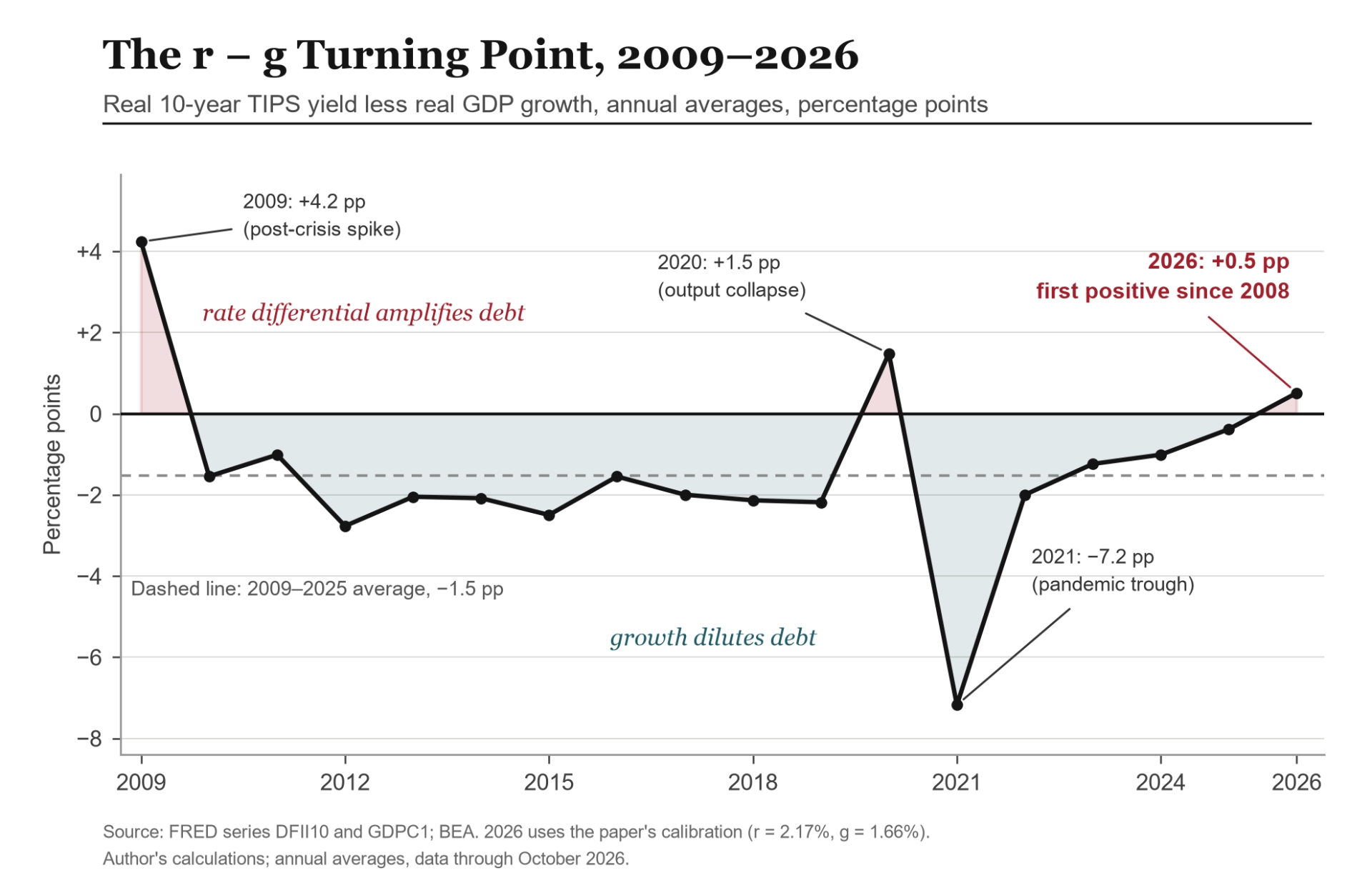
Figure 1. The r − g turning point, 2009–2026.The differential was negative in every year from 2010 to 2025 except 2020, when output collapsed; in 2026 it turned positive for the first time since 2008.

图1. r − g 转折点，2009–2026年。从2010年到2025年，除 2020 年产出大幅萎缩外，该差值在每一年都是负数；2026年，它自2008年以来首次转为正值。

Source: FRED series DFII10 and GDPC1; BEA. 2026 uses the calibration in Section 4.2 (r = 2.17%, g = 1.66%). Author's calculations; annual averages, data through October 2026.

来源：FRED 序列 DFII10 和 GDPC1；BEA。2026年使用第4.2节中的校准(r = 2.17%, g = 1.66%)。作者计算；年度平均值，数据截至2026年10月。

5.3 The Required Primary Surplus and the Fiscal Gap

5.3 所需基本盈余与财政缺口

Under Equation 3, s* = (r − g) × d. With r − g at approximately +0.7%—using a value near the 2026 calibration—and d at 101%, the primary surplus required for stabilization is +0.71% of GDP. Even if the stabilization target is reduced to the IMF benchmark of 85%, a surplus of approximately +0.6% is still required. The actual primary balance is −2.6% of GDP, a deficit. The gap between the actual balance and the +0.71% stabilization point is therefore approximately 3.3 percentage points. Under the current parameters, the direction of U.S. fiscal policy (expansion) is the opposite of the direction required for stabilization (consolidation).

根据方程3，s* = (r − g) × d。当 r − g 约为+0.7%（使用接近2026年校准的值）且 d 为101%时，稳定所需的基本盈余为 GDP 的+0.71%。即使将稳定目标降低到 IMF 的85%基准，仍然需要约+0.6%的盈余。实际基本余额为 GDP 的−2.6%，是赤字。因此，实际余额与+0.71%稳定点之间的缺口约为3.3个百分点。在当前参数下，美国财政政策的方向（扩张）与稳定所需的方向（整顿）相反。

5.4 Scenario Analysis: Divergence Under Current Policy

5.4 情景分析：当前政策下的发散

Starting from d = 101% in 2026, Equation 1 is iterated across five scenarios, with parameters held constant throughout.

从2026年的 d = 101% 开始，方程1在五种情景下迭代，参数始终保持恒定。

Note: Paths iterate Equation 1 (d′ = d × (1 + r)/(1 + g) − s) annually from d = 101% in 2026. Current policy holds the 2026 calibration (r − g = +0.51 percentage point, s = −2.6%); the neutral and moderate-consolidation scenarios keep r − g = +0.51 and set s = −1.82% and −0.20%. The return-to-low-rates scenario holds s = −2.6% and sets r − g = −2.56 points. The CBO baseline column reports the CBO projection quoted in Section 5.1, not a model iteration.

注：路径从2026年的 d = 101% 开始每年迭代方程1 （d′ = d × (1 + r)/(1 + g) − s）。当前政策保持2026年校准(r − g = +0.51个百分点,s = −2.6%)；中性和适度财政整顿情景保持 r − g = +0.51，并设置 s = −1.82% 和 −0.20%。回归低利率情景保持 s = −2.6%，并设置 r − g = −2.56点。CBO 基线一列报告第 5.1 节引用的 CBO 预测，而非模型迭代。

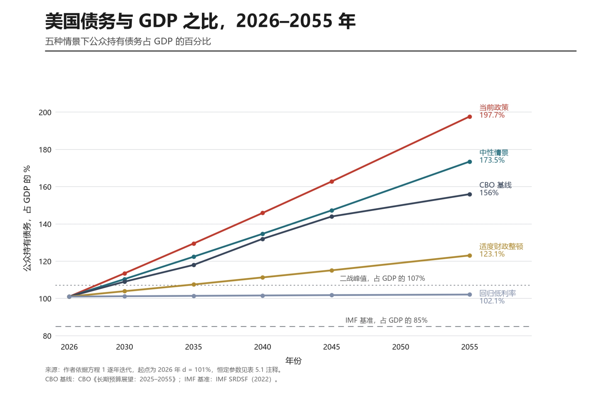
The implication is clear: the debt ratio can be anchored only if interest rates fall below growth again—the "return to low rates" scenario, in which the ratio stabilizes near 102%—or if substantial fiscal consolidation is implemented, with the "moderate consolidation" scenario bringing the ratio down to 123% by 2055. Under current policy and the neutral assumptions, the ratio reaches approximately 198% or 173.5% of GDP in 2055, respectively, well above the CBO baseline of 156%, with no convergence along the way.

结论是明确的：只有在利率再次低于增长率的情况下——“回归低利率”情景，比率稳定在102%附近——或者实施大规模财政整顿，“适度财政整顿”情景到2055年将比率降至123%，债务比率才能锚定。在当前政策和中性假设下，比率在2055年分别达到约198%或173.5%的 GDP，远高于 CBO 基线的156%，且全程没有收敛。

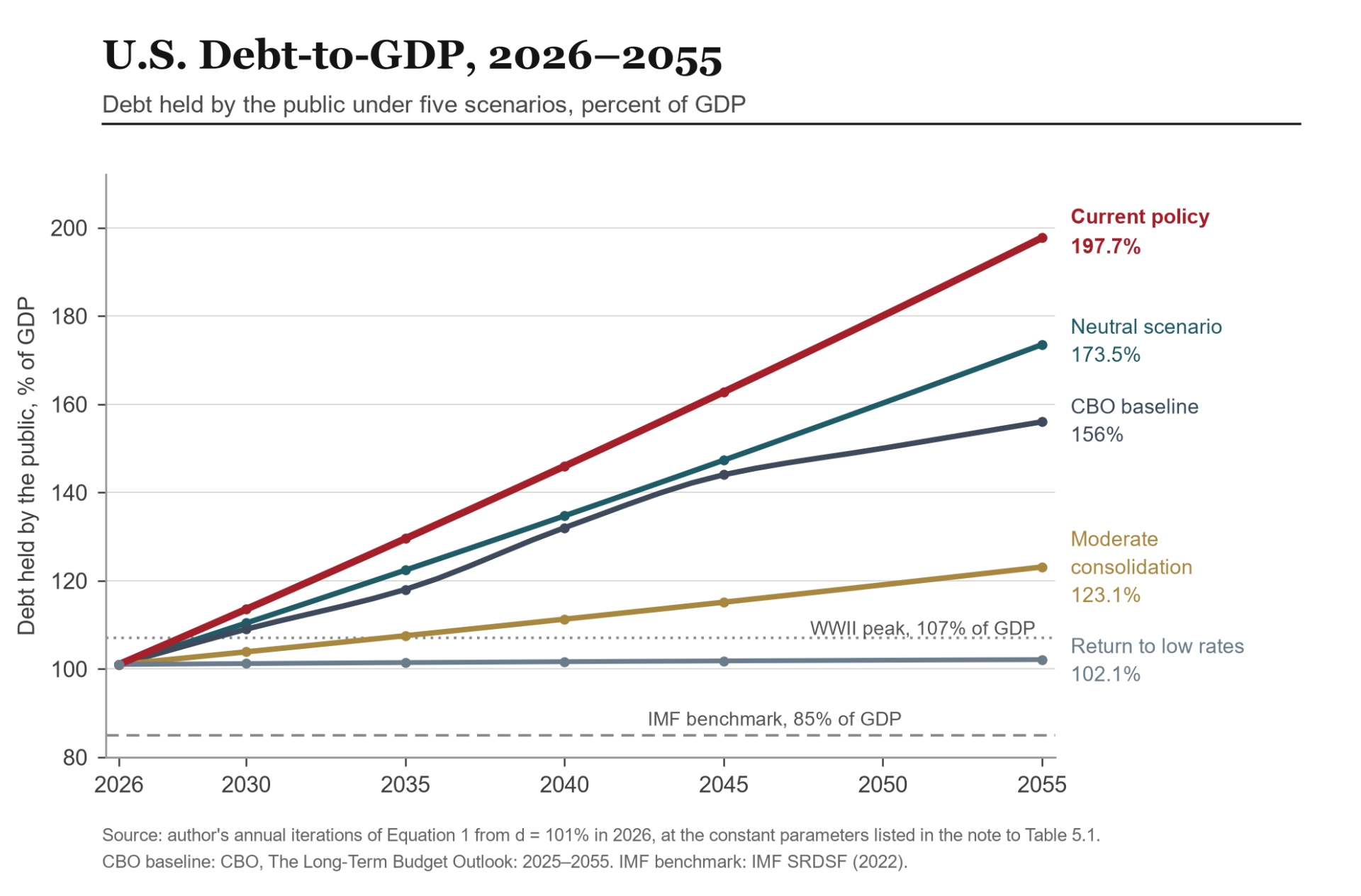
Figure 2. U.S. debt-to-GDP under five scenarios, 2026–2055. Debt held by the public as a percent of GDP, starting from 101% in 2026; each path iterates Equation 1 annually with the constant parameters listed in the note to Table 5.1. The IMF's 85% benchmark and the 1946 peak on this measure (107%) are shown for reference.

图2. 五种情景下的美国债务/GDP，2026–2055年。公众持有的债务占 GDP 的百分比，从2026年的101%开始；每条路径使用表5.1注释中列出的恒定参数每年迭代方程1。IMF 的85%基准和1946年该指标的峰值（107%）一并标示以供参考。

Source: author's annual iterations of Equation 1; CBO, The Long-Term Budget Outlook: 2025–2055, for the baseline. IMF benchmark: IMF SRDSF (2022).

来源：作者对方程1的年度迭代；CBO，《长期预算展望：2025–2055》，用于基线。IMF 基准：IMF SRDSF (2022)。

5.5 The Stability Diagram: The United States Is in the Divergence Region

5.5 稳定性图：美国处于发散区域

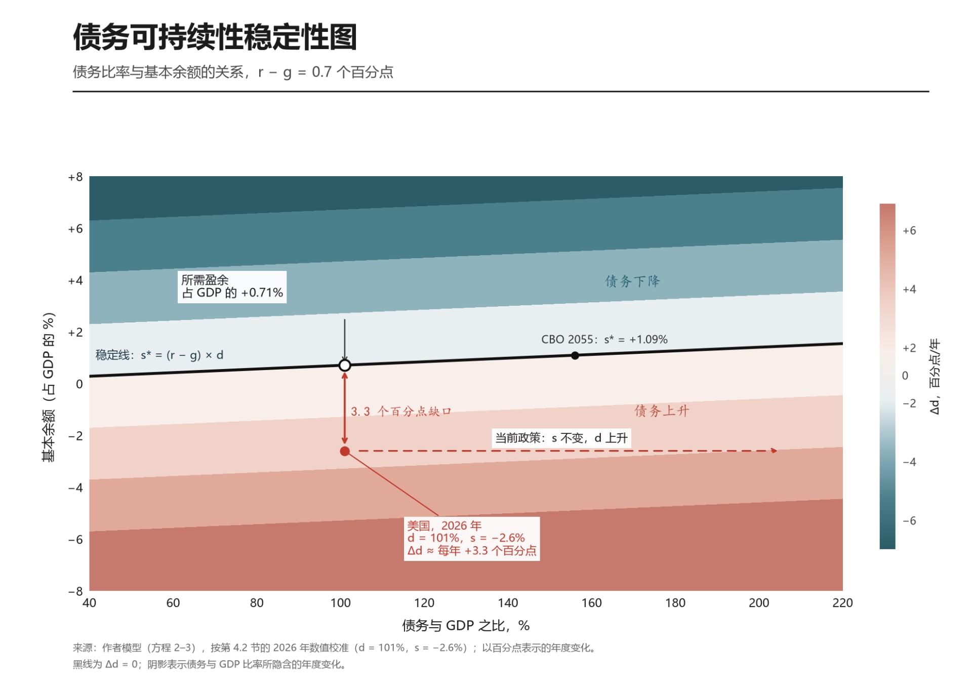
Equation 2 can be used to construct a stability diagram in the (d, s) plane. The stability line, s* = (r − g) × d, using r − g = +0.7%, divides the plane into two regions: above the line, the debt ratio declines; below it, the ratio rises. The U.S. position in 2026 is (d = 101, s = −2.6), on a contour corresponding to an annual increase of approximately 3 percentage points. Under the paper's current parameters, the United States is therefore in the divergence region.

方程2可用于在 (d, s) 平面上构建稳定性图。稳定线 s* = (r − g) × d，使用 r − g = +0.7%，将平面分为两个区域：在线上方，债务比率下降；在线下方，比率上升。美国2026年的位置是 (d = 101, s = −2.6)，位于对应年增长约3个百分点的等值线上。因此，在本文当前参数下，美国处于发散区域。

To enter the declining-debt region, the primary balance would need to improve from −2.6% to above +0.7% of GDP—an adjustment of approximately 3.3 percentage points. The stability line is a knife-edge: a deviation below it produces divergence. This illustrates why even a modest fiscal deterioration can be amplified rapidly when debt is high and r − g is positive.

要进入债务下降区域，基本余额需要从 GDP 的−2.6%改善到+0.7%以上——调整幅度约3.3个百分点。稳定线具有刀刃性质：低于它的偏离即导致发散。这说明了为什么当债务高企且 r − g 为正时，即使是适度的财政恶化也会迅速放大。

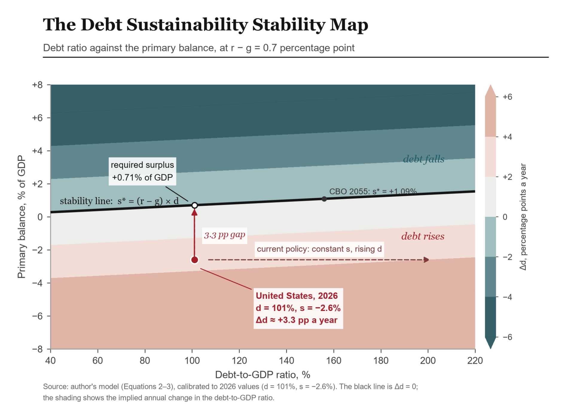
Figure 3. The debt sustainability stability map.Shading shows the annual change in the debt-to-GDP ratio implied by Δd ≈ (r − g) × d − s at r − g = 0.7 percentage point; the black line marks the primary balance that holds the ratio constant. The United States in 2026 sits 3.3 percentage points below that line, on a path that adds roughly 3.3 points a year.

图3. 债务可持续性稳定图。阴影显示在 r − g = 0.7个百分点时，Δd ≈ (r − g) × d − s 所隐含的债务/GDP 比率的年度变化；黑线标记保持比率恒定的基本余额。2026年的美国位于该线下方3.3个百分点处，处于每年增加约3.3点的路径上。

Source: author's model (Equations 2–3), calibrated to the 2026 values in Section 4.2 (d = 101%, s = −2.6%); annual changes in percentage points.

来源：作者的模型（方程2–3），校准到第4.2节中的2026年值(d = 101%, s = −2.6%)；以百分点表示的年度变化。

5.6 Benchmarks and Comparisons

5.6 基准与比较

International benchmarks and model-derived reference points provide a common yardstick for assessing sustainability. On the measures cited in this paper, current U.S. debt exceeds most of the comparison benchmarks.

国际基准和模型衍生的参考点提供了评估可持续性的共同标尺。按照本文引用的指标，当前美国债务超过了大多数比较基准。

6. Conclusions and Policy Implications

6. 结论与政策含义

6.1 Main Findings

6.1 主要发现

First, the sustainability signal has turned adverse. In 2026, r − g turned positive for the first time since 2008, reaching +0.51 percentage point. The United States has moved beyond the "low-interest-rate utopia," and debt dynamics are shifting from growth-driven dilution toward interest-rate-driven amplification.

第一，可持续性信号已转为不利。2026年，r − g 自2008年以来首次转为正值，达到+0.51个百分点。美国已经走出“低利率乌托邦”，债务动态正在从增长驱动的稀释转向利率驱动的放大。

Second, the fiscal gap is approximately 3.3 percentage points. The primary surplus required for stabilization is +0.71% of GDP, while the actual primary balance is a deficit of 2.6%. The fiscal trajectory is moving in the opposite direction from the one required to stabilize the market's debt dynamics.

第二，财政缺口约为3.3个百分点。稳定所需的基本盈余为 GDP 的+0.71%，而实际基本余额为2.6%的赤字。财政轨迹正朝着与稳定市场债务动态所需方向相反的方向移动。

Third, the projected path points toward divergence. Under current-policy and neutral assumptions, debt held by the public reaches approximately 198% or 173.5% of GDP, respectively, by 2055. Even the CBO baseline reaches 156%. All three outcomes are well above the World War II peak and the IMF benchmark, with no convergence over the next three decades. The stability diagram places the United States in the divergence region, with the debt ratio rising by approximately 3 percentage points per year.

        第三，预测路径指向发散。在当前政策和中性假设下，到2055年公众持有的债务分别达到 GDP 的约198%或173.5%。即使是 CBO 基线也达到156%。所有三种结果都远高于二战峰值和 IMF 基准，未来三十年内没有收敛。稳定性图将美国置于发散区域，债务比率每年上升约3个百分点。

6.2 Policy Implications

6.2 政策含义

The need for fiscal consolidation—and its political cost.Under Bohn's (1998) fiscal reaction-function framework, divergence can be reversed only if the primary surplus rises as the debt ratio increases (β > 0). A fiscal gap of 3.3 percentage points implies substantial spending reductions or tax increases. The political resistance to such measures is one of the largest sources of uncertainty.

财政整顿的必要性——及其政治成本。根据 Bohn(1998)的财政反应函数框架，只有在基本盈余随着债务比率增加而上升时(β > 0)，发散才能逆转。3.3个百分点的财政缺口意味着大幅削减支出或增税。对此类措施的政治阻力是最大的不确定性来源之一。

The interest-rate path is another critical determinant.The scenario analysis indicates that a return to low rates—supported by demand for safe assets, financial repression, or flight-to-safety flows during a recession—could stabilize the debt ratio near 100%. Monetary policy is therefore as important as fiscal policy, particularly the ability to maintain lower real interest rates without triggering an uncontrolled rise in inflation.

利率路径是另一个关键决定因素。情景分析表明，回归低利率——由对安全资产的需求、金融抑制或衰退期间的避险资金流动支撑——可以将债务比率稳定在100%附近。因此，货币政策与财政政策同样重要，特别是在不引发失控通胀的情况下维持较低实际利率的能力。

Preserving structural buffers.The United States' "exorbitant privilege" and the global demand for safe assets distinguish it from emerging-market borrowers. Preserving the dollar's and U.S. Treasury securities' reserve-asset status is equivalent to maintaining a low-cost funding channel supported by global capital. This remains an institutional safeguard against a debt crisis.

保持结构性缓冲。美国的“过度特权”和全球对安全资产的需求使其有别于新兴市场借款人。保持美元和美国国债的储备资产地位相当于维持一个由全球资本支持的低成本融资渠道。这仍然是防范债务危机的制度保障。

6.3 Risks and Uncertainties

6.3 风险与不确定性

The projections rely on constant-parameter assumptions. In practice, at least three external shocks could materially alter the conclusions.

预测依赖于恒定参数假设。在实践中，至少有三种外部冲击可能实质性地改变结论。

The first is an inflation shock. Unexpected inflation could reduce real interest rates and dilute the debt ratio through a financial-repression channel, but at the cost of central-bank credibility and potentially the dollar's international standing.

第一种是通胀冲击。意外通胀可以通过金融抑制渠道降低实际利率并稀释债务比率，但代价是中央银行公信力以及可能的美元国际地位。

The second is the crystallization of contingent liabilities (Equation 10), which could produce a one-off increase in debt of 5%–15% of GDP—for example, through a major financial-sector rescue or a larger-than-expected shortfall in social insurance programs.

第二种是或有负债的显性化（方程10），这可能产生 GDP 5%-15%的一次性债务增加——例如，通过重大金融部门救助或社会保险计划中超出预期的缺口。

The third is a structural decline in demand for safe assets, including a shift away from the dollar. Such a change would raise term premiums and r, accelerating debt divergence.

第三种是对安全资产需求的结构性下降，包括减少对美元依赖的转向。这种变化将提高期限溢价和 r，加速债务发散。

The projections should therefore be understood as mechanism-based scenarios, not point forecasts. Their value lies in showing that, as the r − g dividend fades, the United States can no longer rely on growth alone to dilute its debt burden. The policy choice shifts toward either active fiscal consolidation or institutional mechanisms that suppress real interest rates—and neither path is painless.

因此，应将预测理解为基于机制的情景，而非点预测。其价值在于表明，随着 r − g 红利消退，美国不能再仅依靠增长来稀释其债务负担。政策选择转向主动财政整顿或抑制实际利率的制度机制——而两条路径均需付出代价。